Introduction
So far in this series of articles we started off building a basic model for predicting football results using two independent Poisson variables inspired by M. J. Maher. This simple model worked surprisingly well, but had some issues correctly predicting low scores and draws due to the independence of the two Poissons.
In the second part of the series, we used ideas from Dixon and Coles to effectively add some dependance back in to our model via rho, which helped improve its performance with those tricky low scores and draws. We also added in a decay weighting to the data so older fixtures were considered less important that more recent ones when fitting the model.
Next, we're going to implement Baio and Blangiardo's Bayesian hierarchical model to see how well that performs compared with our models so far.
If you've not read through those previous articles yet, I suggest starting there first as it will provide you with the background to what we're doing here.
Let's get started!
The Data
The aim of the model we're building is to predict the number of goals each football (soccer) team will score when they play each other. As always, let's start off by downloading some historical fixtures from football-data.co.uk. Baio and Blangiardo's publication uses the Italian Serie A but we're going to see how their model fares on the English Premier League.
The code below uses the penaltyblog python package to download three season's worth of data into a pandas dataframe and renames the columns to match the syntax used by Baio and Blangiardo. The home_team and away_team columns contain the team names, and yg1 and yg2 are the number of goals scored by the home team and away team, respectively. We've also kept the date column, and the result of each fixture.
import pandas as pd
import penaltyblog as pb

fixtures = pd.concat(
    [
        pb.footballdata.fetch_data("england", 2018, 0),
        pb.footballdata.fetch_data("england", 2019, 0),
        pb.footballdata.fetch_data("england", 2020, 0),
    ]
).rename(
    columns={
        "HomeTeam": "home_team",
        "AwayTeam": "away_team",
        "FTHG": "yg1",
        "FTAG": "yg2",
        "FTR": "result"
    }
)

fixtures = fixtures[["Date", "home_team", "away_team", "yg1", "yg2", "result"]]

fixtures.head()
| Date | home_team | away_team | yg1 | yg2 | result | |
|---|---|---|---|---|---|---|
| 0 | 2018-08-10 | Man United | Leicester | 2 | 1 | H |
| 1 | 2018-08-11 | Bournemouth | Cardiff | 2 | 0 | H |
| 2 | 2018-08-11 | Fulham | Crystal Palace | 0 | 2 | A |
| 3 | 2018-08-11 | Huddersfield | Chelsea | 0 | 3 | A |
| 4 | 2018-08-11 | Newcastle | Tottenham | 1 | 2 | A |
We need to give each team a unique ID, as this will make the data easier to handle later on.
import numpy as np

n_teams = len(fixtures["home_team"].unique())

teams = (
    fixtures[["home_team"]]
    .drop_duplicates()
    .sort_values("home_team")
    .reset_index(drop=True)
    .assign(team_index=np.arange(n_teams))
    .rename(columns={"home_team": "team"})
)

df = (
    fixtures.merge(teams, left_on="home_team", right_on="team")
    .rename(columns={"team_index": "hg"})
    .drop(["team"], axis=1)
    .merge(teams, left_on="away_team", right_on="team")
    .rename(columns={"team_index": "ag"})
    .drop(["team"], axis=1)
    .sort_values("Date")
)

df.head()
| Date | home_team | away_team | yg1 | yg2 | result | hg | ag | |
|---|---|---|---|---|---|---|---|---|
| 0 | 2018-08-10 | Man United | Leicester | 2 | 1 | H | 15 | 12 |
| 505 | 2018-08-11 | Watford | Brighton | 2 | 0 | H | 21 | 3 |
| 932 | 2018-08-11 | Bournemouth | Cardiff | 2 | 0 | H | 2 | 5 |
| 881 | 2018-08-11 | Huddersfield | Chelsea | 0 | 3 | A | 10 | 6 |
| 290 | 2018-08-11 | Fulham | Crystal Palace | 0 | 2 | A | 9 | 7 |
The hg column now contains the ID for the home team and the ag column is the ID for the away team. So for example, Manchester United are team 15 and Brighton are team 3.
Next, we split the data in to a train and test data set. The train data is used to fit the model, while we hold back 250 fixtures to test the model's performance on. We also extract the team IDs and goals scored from the train data into numpy arrays as it makes them a little easier to work with later on.
TEST_SIZE = 250
train = df.iloc[:-TEST_SIZE]
test = df.iloc[-TEST_SIZE:]

goals_home_obs = train["yg1"].values
goals_away_obs = train["yg2"].values
home_team = train["hg"].values
away_team = train["ag"].values
Defining the Model
The model itself is the same as the previous Poisson models we've created. We are still assuming that the number of goals a team scores is a function of their attack strength combined with the opposition's defence strength. In other words, teams with better attacks should score more and teams with worse defences should concede more. We also include home field advantage.
So the model still looks like this:
goals_home = home_advantage + home_attack + defence_away
goals_away = away_attack + defence_home
Where it changes this time though is how we implement it as we're going Bayesian...
Bayesian Statistics
Bayesian statistics is a very deep subject area, which I would certainly not be able to do justice to here so if you really want to dig into the details then I whole heartedly recommend reading Statistical Rethinking by Richard McElreath and Doing Bayesian Data Analysis: A Tutorial with R, JAGS, and Stan by John Kruschke. I'm by no means an expert in the subject but I've learnt a huge amount from these two books alone.
But at a very high level for us building our model (and apologies to any real Bayesians reading this), the biggest difference here using a Bayesian approach is that we get a distribution of values for each model parameter rather than the single values we had previously.
Bayesian modelling also lends itself well to using a technique known as hierarchical modeling (also known as multilevel modelling or mixed-effects modelling). This allows us to account for relationships between variables by considering them to come from a common distribution.
What that means for us is that we can avoid the problems the independent Poisson variables caused in our previous two models. By using a hierarchical model containing two conditionally independent Poisson variables, correlation between the two is naturally taken into account as our observable variables are mixed at an upper level in the model.
In other words, we don't need to bother applying the Dixon and Coles adjustment to our model's output anymore. Hurrah!
Building the Model
We're using the awesome PyMC3 library in Python to build our model, as shown below.
The home parameter refers to the advantage teams get from playing at home. This is a fixed effect that assumes the advantage is constant across all teams and across the entire time the dataset covers. We assign an uninformative flat prior to it, meaning that its value comes from a uniform distribution ranging anywhere from -infinity to +infinity.
atts and defs represent each team's attack and defence ratings. Although each team has its own unique ratings, they are estimated from a common distribution. Whilst each football team is clearly different to each other, they are all playing in the same league so we make the reasonable assumption that their ratings come from the same distribution. This allows us to pool related data together, which can often improve model estimates. Our prior here is that the ratings are normally distributed.
It's worth pointing out that we are subtracting the mean ratings from both the attack and defence ratings to ensure identifiability. There are countless combinations of parameters that could potentially give us the same results so this forces the model to give us a reproducible output and keeps the parameters in a realistic range.
The final chunk of code, where we calculate home_theta and away_theta, looks very similar to our previous models. We just sum up the ratings and home advantage to calculate the goal expectancy for each team and apply that to a Poisson distribution.
import pymc3 as pm
import theano.tensor as tt

with pm.Model() as model:
    # home advantage
    home = pm.Flat("home")

    # attack ratings
    tau_att = pm.Gamma("tau_att", 0.1, 0.1)
    atts_star = pm.Normal("atts_star", mu=0, tau=tau_att, shape=n_teams)

    # defence ratings
    tau_def = pm.Gamma("tau_def", 0.1, 0.1)
    def_star = pm.Normal("def_star", mu=0, tau=tau_def, shape=n_teams)

    # apply sum zero constraints
    atts = pm.Deterministic("atts", atts_star - tt.mean(atts_star))
    defs = pm.Deterministic("defs", def_star - tt.mean(def_star))

    # calulate theta
    home_theta = tt.exp(home + atts[home_team] + defs[away_team])
    away_theta = tt.exp(atts[away_team] + defs[home_team])

    # goal expectation
    home_points = pm.Poisson("home_goals", mu=home_theta, observed=goals_home_obs)
    away_points = pm.Poisson("away_goals", mu=away_theta, observed=goals_away_obs)
Fitting the Model
Drum roll... now we fit the model by calling PyMC3's sample function. We're sampling 2000 times across six chains, which gives us 12,000 samples in total to play with. We've also set tune to 1000, which means each chain will throw away 1000 samples before starting as these initial samples can sometimes be more uncertain.
with model:
    trace = pm.sample(2000, tune=1000, cores=6, return_inferencedata=False)
Let's check how well the model has done by looking at it's fitted parameters. We'll start off with the home advantage.
with model:
    pm.plot_trace(trace, var_names=["home"]);
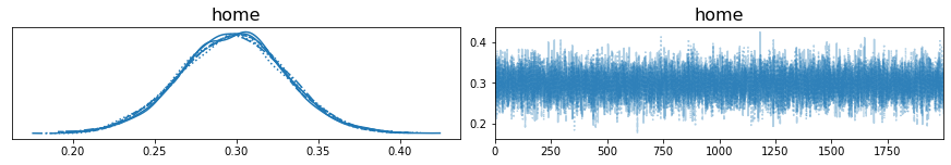
As I mentioned above, with Bayesian models we get a distribution of possible parameter values rather than a single point estimate. Reassuringly, we've got a smooth curve here centred somewhere around 0.3, with is pretty close to the home advantage we saw for our Poisson models - our Dixon and Coles model in the last article gave us a value of 0.294.
We can also take a look at the attack and defence ratings.
with model:
    pm.plot_trace(trace, var_names=["atts", "defs"]);
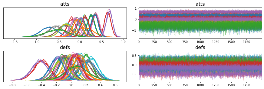
Again, we've got nice looking curves which is reassuring but that looks a little busy with 20 different attack and defence curves so let's replot the data a little differently.
import arviz as az
import matplotlib.pyplot as plt

atts = (
    pd.DataFrame(az.stats.hdi(trace["atts"]), columns=["lower_hdi", "upper_hdi"])
    .assign(median=np.quantile(trace["atts"], 0.5, axis=0))
    .merge(teams, left_index=True, right_on="team_index")
    .drop(["team_index"], axis=1)
    .rename(columns={"team": "Team"})
    .assign(lower=lambda x: x["median"] - x["lower_hdi"])
    .assign(upper=lambda x: x["upper_hdi"] - x["median"])
    .sort_values("median", ascending=True)
)

plt.errorbar(
    atts["median"],
    atts["Team"],
    xerr=(atts[["lower", "upper"]].values).T,
    fmt="o",
)
defs = (
    pd.DataFrame(az.stats.hdi(trace["defs"]), columns=["lower_hdi", "upper_hdi"])
    .assign(median=np.quantile(trace["defs"], 0.5, axis=0))
    .merge(teams, left_index=True, right_on="team_index")
    .drop(["team_index"], axis=1)
    .rename(columns={"team": "Team"})
    .assign(lower=lambda x: x["median"] - x["lower_hdi"])
    .assign(upper=lambda x: x["upper_hdi"] - x["median"])
    .sort_values("median", ascending=False)
)

plt.errorbar(
    defs["median"],
    defs["Team"],
    xerr=(defs[["lower", "upper"]].values).T,
    fmt="o",
)
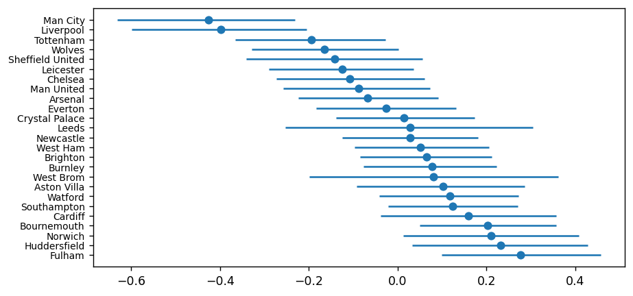
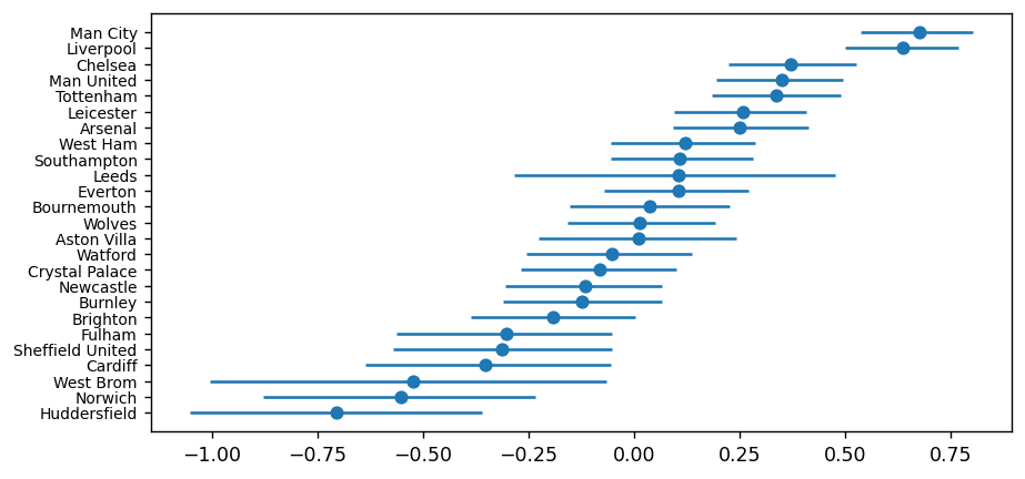
These last two plots show us the median value for each team's attack and defence rating (the dot in the middle), plus the high density interval or HDI (the horizontal line). You can think of the HDI as being the Bayesian equivalent to a 95% confidence interval.
Again, the results pass the eye test - Manchester City and Liverpool have the highest attack rating (meaning the model thinks they score the most goals) and the lowest defence rating (meaning they concede the fewest goals). Plus, we have Huddersfield and Norwich being terrible at both ends of the pitch.
The width of the HDI represents the model's uncertainty for the parameter, where the wider the bar the more uncertain we are of the parameter's true value. Typically, it tends to be wider here for teams that have been promoted / relegated as we have less data available for them in the data set.
Predicting Results
So far, so good. We've fit our model and its parameters look feasible so the next stage is to predict some results.
Things are slightly different with this model though as we don't have a specific value for each of our parameters. Instead, we have a distribution of values - in fact, we have 12,000 values for each parameter (remember that's how many samples we got back when we fit the model).
To simplify things though we'll just collapse our distributions down to a single value by taking the average of each parameter, which we can then use to calculate the goal expectation in a similar way to how we did it for our previous Poisson models.
This makes me sad though as one of the major advantages of Bayesian models is having these distributions so it seems a shame to throw them away and just keep their average. However, I seem to get the same results doing this compared with other approaches I've tried so let's go with it.
The chunk of code below shows how to do this. The first few lines just pull out the average parameters from the model's output for a given home and away team. We then use these values to calculate the goal expectation. If you've read the previous two articles in this series then there's nothing particularly unexpected here.
def goal_expectation(trace, home_team_id, away_team_id):
    # get parameters
    home = np.mean(trace["home"])
    atts_home = np.mean([x[home_team_id] for x in trace["atts"]])
    atts_away = np.mean([x[away_team_id] for x in trace["atts"]])
    defs_home = np.mean([x[home_team_id] for x in trace["defs"]])
    defs_away = np.mean([x[away_team_id] for x in trace["defs"]])

    # calculate theta
    home_theta = np.exp(home + atts_home + defs_away)
    away_theta = np.exp(atts_away + defs_home)

    # return the average per team
    return home_theta, away_theta
We then just need to pass in the model's output and the relevant team IDs to get our predicted number of goals. Let's give it a try for Manchester City Vs Manchester United.
goal_expectation(trace, 14, 15)

(2.40817399509211, 0.9015500181975004)
As a Manchester City fan, this makes me happy as it has City winning by 2.4 goals to 0.9 goals :)
Let's flip it around and have Manchester United as the home team.
goal_expectation(trace, 15, 14)

(1.2138865328696127, 1.7885438632930635)
Nice, even without the home advantage Manchester City is still winning.
Is Our Bayesian Model Any Good?
Now it's time to assess whether these predictions are actually any good or not. We'll do this by predicting the probability of home win / draw / away win for each fixture in our test data set and compare it to what actually happened using Rank Probability Scores to measure the error. I explained why we use Rank Probability Scores in the last article so take a look here if you want to know more.
To do this, we're going to need to convert our predicted score lines to win / draw / loss probabilities. This is exactly the same as how we did it in the previous articles. We just use the Poisson distribution to get the probability of scoring 0-10 goals for each team, then take the outer product of the two to get the probabilities for each possible scoreline.
The sum of the upper triangle of the resulting matrix is the probability an away win, the sum of the diagonal is the probability of a draw and the sum of the lower triangle is the probability of a home win.
from scipy.stats import poisson

def win_draw_loss(home_expectation, away_expectation, max_goals=10):
    h = poisson.pmf(range(max_goals+1), home_expectation)
    a = poisson.pmf(range(max_goals+1), away_expectation)
    m = np.outer(h, a)

    home = np.sum(np.tril(m, -1))
    away = np.sum(np.triu(m, 1))
    draw = np.sum(np.diag(m))

    return home, draw, away
And here's the function to calculate the Rank Probability Score of our model on our test data. It's pretty simple, we just loop through the fixtures and decide whether the actual result was a home win, draw or away win. We then get the probabilities for each outcome from our model and calculate the Rank Probability Score for our predictions versus what actually happened. Finally, we return the average error.
def calculate_rps(df):
    rps = list()
    for idx, row in df.iterrows():
        if row["result"] == "H":
            outcome = 0
        elif row["result"] == "D":
            outcome = 1
        elif row["result"] == "A":
            outcome = 2

        h, a = goal_expectation(trace, row["hg"], row["ag"])
        predictions = win_draw_loss(h, a)

        rps.append(pb.metrics.rps(predictions, outcome))

    return np.mean(rps)
Let's give it a go and see what happens.
calculate_rps(test)

0.21976530250997778
We've got our average error but is this any good or not? Let's run our Dixon and Coles model over the same data and compare the error to see which is best.
def calculate_rps_dc(dc, df):
    rps = list()
    for idx, row in df.iterrows():
        if row["result"] == "H":
            outcome = 0
        elif row["result"] == "D":
            outcome = 1
        elif row["result"] == "A":
            outcome = 2

        predictions = dc.predict(row["home_team"], row["away_team"]).home_draw_away

        rps.append(pb.metrics.rps(predictions, outcome))

    return np.mean(rps)

train["weight"] = pb.poisson.dixon_coles_weights(train["Date"],  0.001)

dc = pb.poisson.DixonColesGoalModel(
    train["yg1"],
    train["yg2"],
    train["home_team"],
    train["away_team"],
    train["weight"]
)

dc.fit()

calculate_rps_dc(dc, test)

0.21589324705157467
Oh dear, the average error for our Bayesian model is actually slightly higher than for our Dixon and Coles model for this particular set of data :(
Why is this?
The first reason is that our Dixon and Coles model has a decay weighting built in to it. This means that it considers more recent data to be more important that older data when estimating the model's parameters. Currently, our Bayesian model lacks this so it considers all data to be equally important.
We know that team's strengths are dynamic and vary over time due to form, injuries, transfers etc so this is definitely a limitation of our current Bayesian approach.
Overshrinkage
The second reason is something called overshrinkage. This a well known problem associated with hierarchical models where more extreme values get pulled back towards the overall average of the data.
For us, it means that the best teams, such as Liverpool and Manchester City, will not appear as strong as they should be whilst the really bad teams, such as Huddersfield, will appear better than they should. Essentially, our parameter estimates get regressed towards the mean, which reduces the model's performance.
Baio and Blangiardo discuss this issue in their publication and propose a solution where by they restructure their model to put teams into one of three different groups - top teams, mid-table teams or bottom teams. The model then uses this grouping within the hierarchical model so that parameters are estimated from a distribution of similar quality teams to try and reduce the overshrinkage.
We've covered a lot of ground in this article already though so I'm going to save digging any further into the overshrinkage for a future blog post.
Conclusions
We've built a Bayesian model using Python and PyMC3 that's capable of predicting football results. Its performance is pretty close to our previous Dixon and Coles model despite being a simpler model in many ways - it doesn't have a decay weighting included yet and it doesn't require the rho adjustment either, plus we've not accounted for the overshrinkage issue - so we've got a pretty good base model here to build on.
Thanks for reading!