tl;dr
- Support Vector Machines provide a viable approach for calculating expected goals
- Forecasting expected goals conceded seems more difficult than expected goals scored
- Expected goals have lots of variability associated with them so calculate confidence intervals rather than just point estimates
Introduction
I've written about expected goals on this website before but I've changed approach recently so I thought I'd write up some of the different ideas I've been playing around with.
My previous expected goals model was very basic. It was essentially a non-linear regression using an exponential decay curve fitted against shot xy coordinates. Sure, there were different curves for foot shots, headed shots etc but that was about as sophisticated as it got.
An alternative approach though is to consider expected goals as a binary problem. Shots either end up in the net and score a goal or they don't. There is no other outcome, no middle ground, no half way, it's either a goal or it's not a goal. So, since this gives us just two distinct outcomes to predict, we can view expected goals as a classification problem rather than regression.
What's the difference? Well, classification and regression are inherently linked but to put it simply classification forecasts whether something will happen where as regression forecasts how much something will happen.
This means we are interested in predicting the probability a shot produces a goal rather than how much of a goal a shot is worth (which is what my previous model did). It may sound a somewhat subtle difference between the two but it opens up the opportunity to use a number of different modelling techniques.
Support Vector Machines
Support vector machines (SVM) are models often used in machine learning for data classification. They have the ability to analyse data sets and identify patterns that can then be used to forecast classes for new data points.
SVMs do this by identifying the hyperplane that separates the different categories within a training data set by the largest margin. Okay, that sounds fairly complex so as a simple example, imagine having a collection of apples and oranges sat on a table top. You could separate the different fruit by drawing a line between them so that all the apples and oranges were on opposite sides of the line. Next, imagine the fruit are now floating at different heights in the air. That simple line we drew before isn't going cut it so instead we slide a sheet of paper between the fruit to separate the apples from the oranges. As we add in more and more dimensions the sheet of paper becomes too simple to represent the separation between the fruit so we move to using a hyperplane.
SVMs also have the added benefits that they can handle non-linear data and calculate probabilities rather than just output binary predictions. So, in terms of expected goals we've got a technique that can handle the non-linearities in the shot distances and provide probabilities of shots resulting in goals. Sounds promising!
The Data
Support Vector Machines rely on a technique known as supervised learning. This means we have to train the model using a set of shots labelled with whether they lead to a goal or not. This training set was created from approximately 30,000 shots taken from the English Premier League's 2012/2013 and 2013/2014 seasons. This included open-play shots taken with head or feet, as well as free kicks and penalties.
The model was then validated using shots taken during the English Premier League's 2014/2015 season. The reason for separating the data out like this is that it helps avoid overfitting and provides a much more realistic estimation of how well the model really works. We want to create a model that generalises well and can forecast future shots. If we test the model on the same data we trained it on then we run the risk of optimising towards noise in the data and creating something that only forecasts well over the dataset it was trained with.
Initial Results
Let's start off simple and see if the preliminary results look feasible. In the test dataset there were 942 goals scored, while the trained SVM predicted 939 goals. This means we're out by just 3 goals, which is around 0.3% of the total. That looks like a pretty good start but we need to be careful here. We could be making really bad forecasts and just be lucky that all the errors are stacking up nicely and masking how bad we are.
We can find out the error by looking at the root mean square error (RMSE). This metric aggregates the differences between the model's forecasts and what actually happened to provide a single value representing the average error we made. For our SVM this came out at 0.269.
On its own this RMSE doesn't really mean much. Is 0.269 good, bad or average? RMSE isn't really meant to be used on its own though, its strength lies in providing a simple metric that can be used to compare the predictive power of different models. So what do we compare with? Well, a recent article on Deadspin criticising expected goals suggested that ignoring shot location and just using the average conversion rate gives equivalent results so let's use that as our baseline to compare against.
This naïve model, which is effectively just measuring total shots, predicted 978 goals for the test data set, with an RMSE of 0.294. So, on both metrics the SVM out performed the baseline meaning we are adding something worthwhile to the predictions.
Are You Certain About That?
So far all the forecasts have been individual point estimates. We can do better than that though and provide a range of values that our expected goals forecast likely falls within.
A common way to do this for SVMs is Bootstrapping. Instead of using our training set to create a single model, we repeatedly resample the shots to create thousands of different combinations of our data and train different SVMs with them. We can then take the average prediction from our set of SVMs as the point estimate and use the distribution of all the individual predictions to calculate a confidence interval representing the uncertainty associated with our forecast.
Doing this with 1,000 SVMs each trained on 30,000 resampled shots gives us our expected goals forecast above of 939 goals, with a 95% confidence interval of 820 - 1057 goals (approximately 12% in either direction, Figure One).
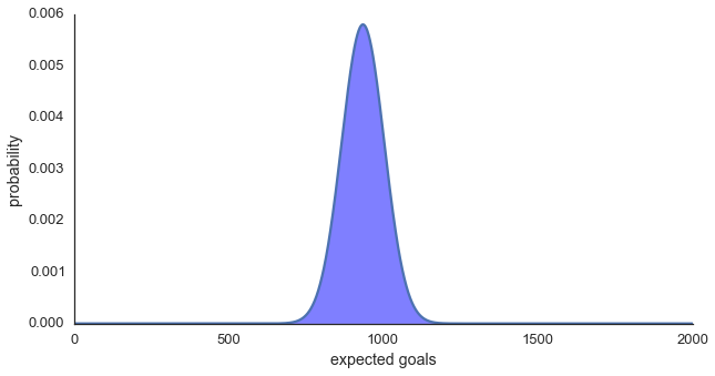
Figure One: Distribution of expected goals
Penalties
Another quick check of the SVM's feasibility is how well it performs on penalties. In the test data set there were 83 penalties taken of which 20 were missed, making a penalty worth 0.76 goals on average. Using the Bootstrapped SVM, a penalty is valued at 0.75 expected goals, with a 95% confidence interval of 0.75 - 0.79. The confidence interval looks pretty narrow and neatly encompasses the expected value so again the our SVM approach looks to be on the right track.
I previously posted an example from my exponential decay model showing that a headed shot from taken from the penalty spot had a value of around 0.08 expected goals. Moving this example to the Bootstrapped SVM gives 0.081 expected goals, with a 95% confidence interval of 0.076 - 0.085. The exponential decay model worked reasonably well at the time (with some limitations) so it's reassuring to see the results are still in line with each other.
Expected Goals By Team
This all looks good so far but we're not generally interested in predicting the total expected goals for a league - expected goals per team are of much more interest. Figure Two below shows expected goals scored versus actual goals scored for the English Premier League 2014/2015 season. The line denotes the linear regression between the two values and the shaded region the 95% confidence interval for the regression. For those interested, the r2 for the regression was 0.822 and the RMSE was 7.21. For comparison, the naïve model had an r2 of 0.707 and an RMSE of 9.16, both of which were inferior to the Bootstrapped SVM.
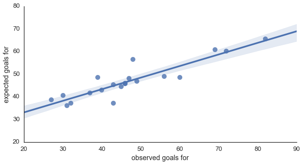
Figure Two: Expected versus actual goals for
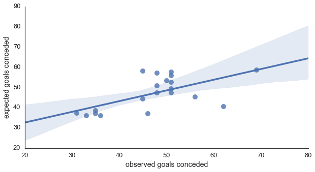
Figure Three below shows the same plot but for expected goals conceded versus actual goals conceded. Notice how much wider the shaded region is, meaning we have much less certainty forecasting goals conceded. This matches what Will Gurpinar-Morgan previously reported (incidentally if you haven't Will's article on expected goals it's well worth a read as he goes into the uncertainty aspect in more detail than I have here). As well as the confidence interval widening, the r2 dropped to 0.521 and the RMSE increased to 16.33. For comparison, the r2 (0.486) and RMSE (20.57) of the naïve model also worsened, and again were inferior to the SVM.
Expected Goals By Player
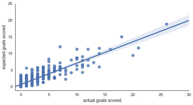
And just for completion, Figure Four shows expected goals versus actual goals at the player level. As expected, since we're slicing the data to a much more granular level, the r2 is slightly lower than for team goals at 0.786, with an RMSE of 1.70. It looks better than I initially expected though as the 95% confidence interval looks surprisingly narrow.
Discussion
This article is already way too long so I'm going to draw it too a close here (congratulations if you made it all the way through!) but I am planning on writing more about expected goals and SVMs in future posts.
The standout points for me though are that SVMs seems a viable approach to calculating expected goals and comfortably outperform the naïve model that ignores shot locations. The SVM model also handles both foot and head shots, as well as free kicks and penalties, which my previous exponential decay model could not.
The fact that expected goals conceded forecasts are so much poorer than those for expected goals scored is intriguing and warrants further study. Presumably, there is some factor having a noticeable impact on whether the defending team concedes that the model does not currently account for and which has less of an impact on whether the attacking team scores.
Finally, since there is a reasonable amount of uncertainty associated with expected goals forecasts I strongly advise calculating confidence intervals rather than just point estimates as it adds much more context to the metric.
Thanks for reading!